Nearest neighbour sweep

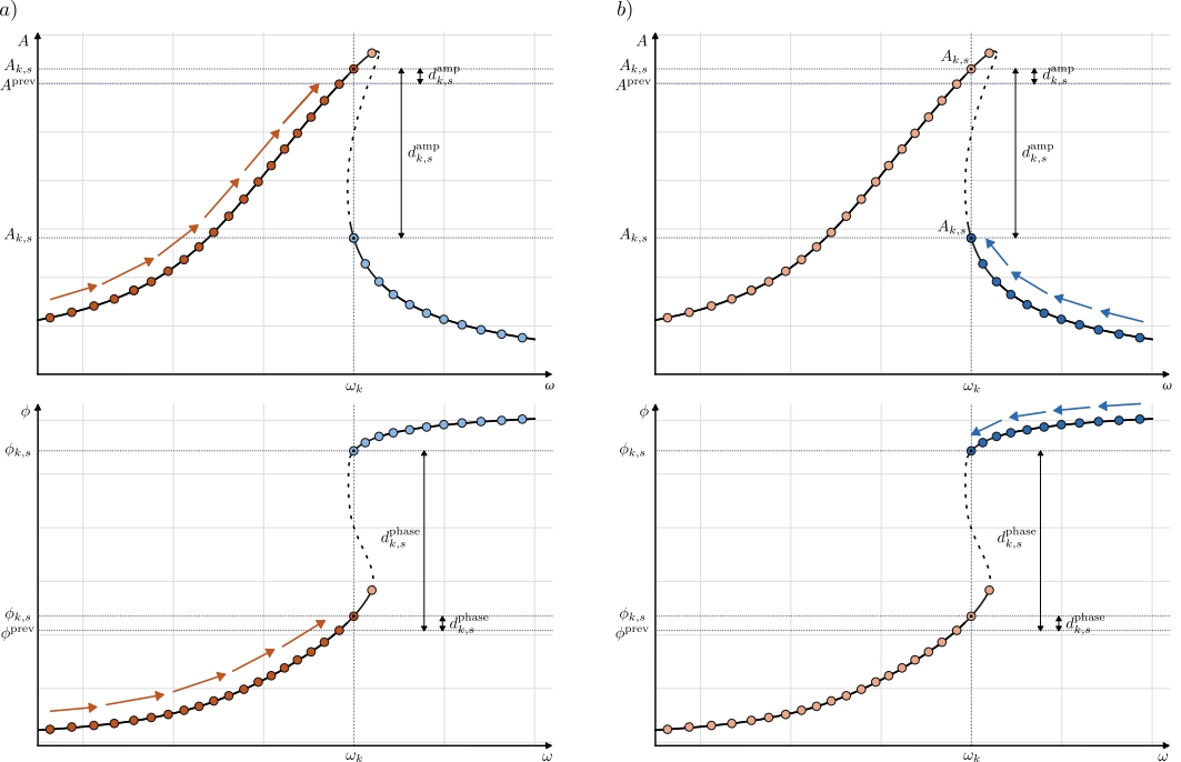
Let the candidate solutions at frequency step \(k\) be indexed by \(s = 1, \dots, N_{\mathrm{seeds}}\), with modal amplitude vector \(\mathbf{A}_{k,s}\) and phase vector \(\boldsymbol{\phi}_{k,s}\). The distance in amplitude to the previously selected solution is defined as

\[ d^{\mathrm{amp}}_{k,s} = \frac{ \sqrt{\frac{1}{M}\sum_{i=1}^{M}\left(A_{k,s,i} - A_i^{\mathrm{prev}}\right)^2} }{ \sqrt{\frac{1}{M}\sum_{i=1}^{M}\left(A_i^{\mathrm{prev}}\right)^2} + \varepsilon }. \]

where \(M\) is the number of response components and \(\varepsilon\) is a small constant introduced to avoid division by zero.

To account for phase wrapping, the phase mismatch is evaluated using a circular distance:

\[ \Delta \phi_{k,s,i} = \arg\!\left(e^{j(\phi_{k,s,i} - \phi_i^{\mathrm{prev}})}\right). \]

The corresponding normalized phase distance is

\[ d^{\mathrm{phase}}_{k,s} = \frac{ \sqrt{\frac{1}{M}\sum_{i=1}^{M}\left(\Delta \phi_{k,s,i}\right)^2} }{\pi}. \]

These two terms are combined into a total cost function

\[ d_{k,s} = d^{\mathrm{amp}}_{k,s} + w_{\phi}\, d^{\mathrm{phase}}_{k,s} + \lambda_{\mathrm{switch}}\, \mathbf{1}_{s \neq s^{\mathrm{prev}}}. \]

where \(w_{\phi}\) controls the relative importance of phase continuity and \(\lambda_{\mathrm{switch}}\) penalizes switching to a different seed than the one selected at the previous step. The indicator function is defined as

\[ \mathbf{1}_{s \neq s^{\mathrm{prev}}} = \begin{cases} 1, & s \neq s^{\mathrm{prev}}, \\ 0, & s = s^{\mathrm{prev}}. \end{cases} \]

The selected solution at frequency step \(k\) is then

\[ s_k = \arg\min_s d_{k,s}. \]

After selection, the reference state is updated according to

\[ \mathbf{A}^{\mathrm{prev}} \leftarrow \mathbf{A}_{k,s_k}, \qquad \boldsymbol{\phi}^{\mathrm{prev}} \leftarrow \boldsymbol{\phi}_{k,s_k}. \]

The sweep is initialized by selecting the medoid of the candidate amplitude vectors at the initial frequency step. In other words, the initial seed is chosen as the candidate whose average distance to all other candidates is minimal. Denoting the candidate amplitude vectors at \(k=0\) by \(\mathbf{A}_{0,s}\), this is written as

\[ s_0 = \arg\min_s \frac{1}{N_{\mathrm{seeds}}} \sum_{r=1}^{N_{\mathrm{seeds}}} d\!\left(\mathbf{A}_{0,s}, \mathbf{A}_{0,r}\right). \]

where \(d(\cdot,\cdot)\) is a distance measure between amplitude vectors. In the present work, the normalized root-mean-square distance is used:

\[ d\!\left(\mathbf{A}_{0,s}, \mathbf{A}_{0,r}\right) = \sqrt{ \frac{1}{M} \sum_{i=1}^{M} \left(A_{0,s,i} - A_{0,r,i}\right)^2 }. \]

This initialization selects a representative candidate among the available responses while ensuring that the starting point corresponds to an actually computed solution.

Overall, this is a greedy selection rule in frequency space. It can produce smooth, experiment-like response paths by minimizing local mismatch in amplitude and phase while discouraging unnecessary seed changes. It is not continuation and does not establish stability, completeness, or physical realizability of every selected path. Interpret it together with multistart coverage and the documented limitations.